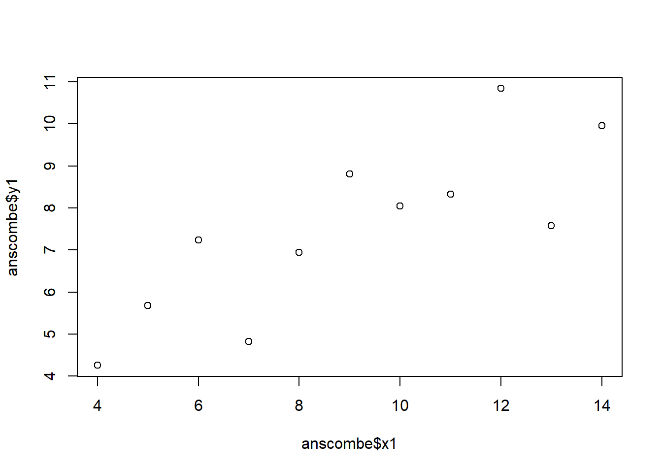
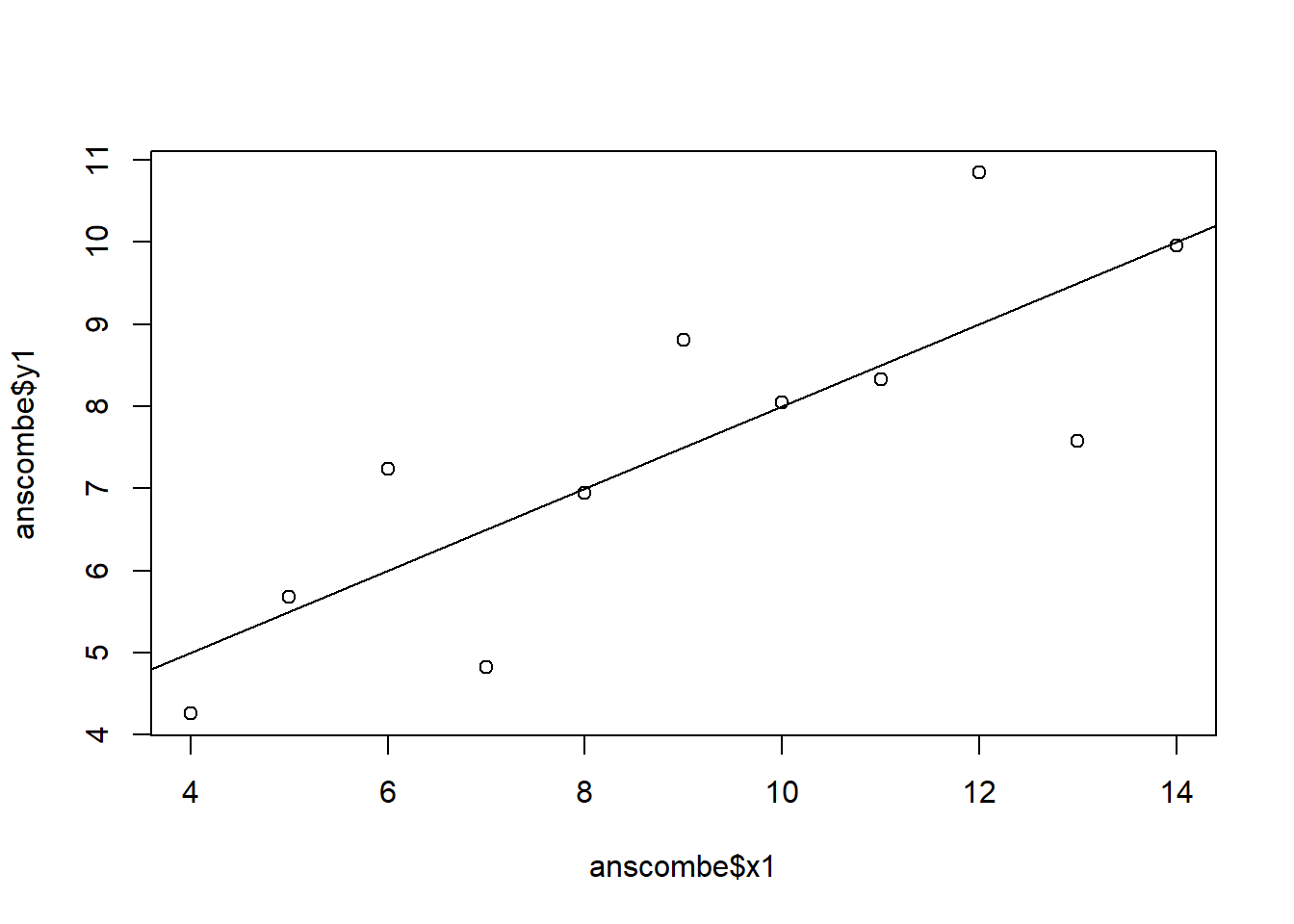
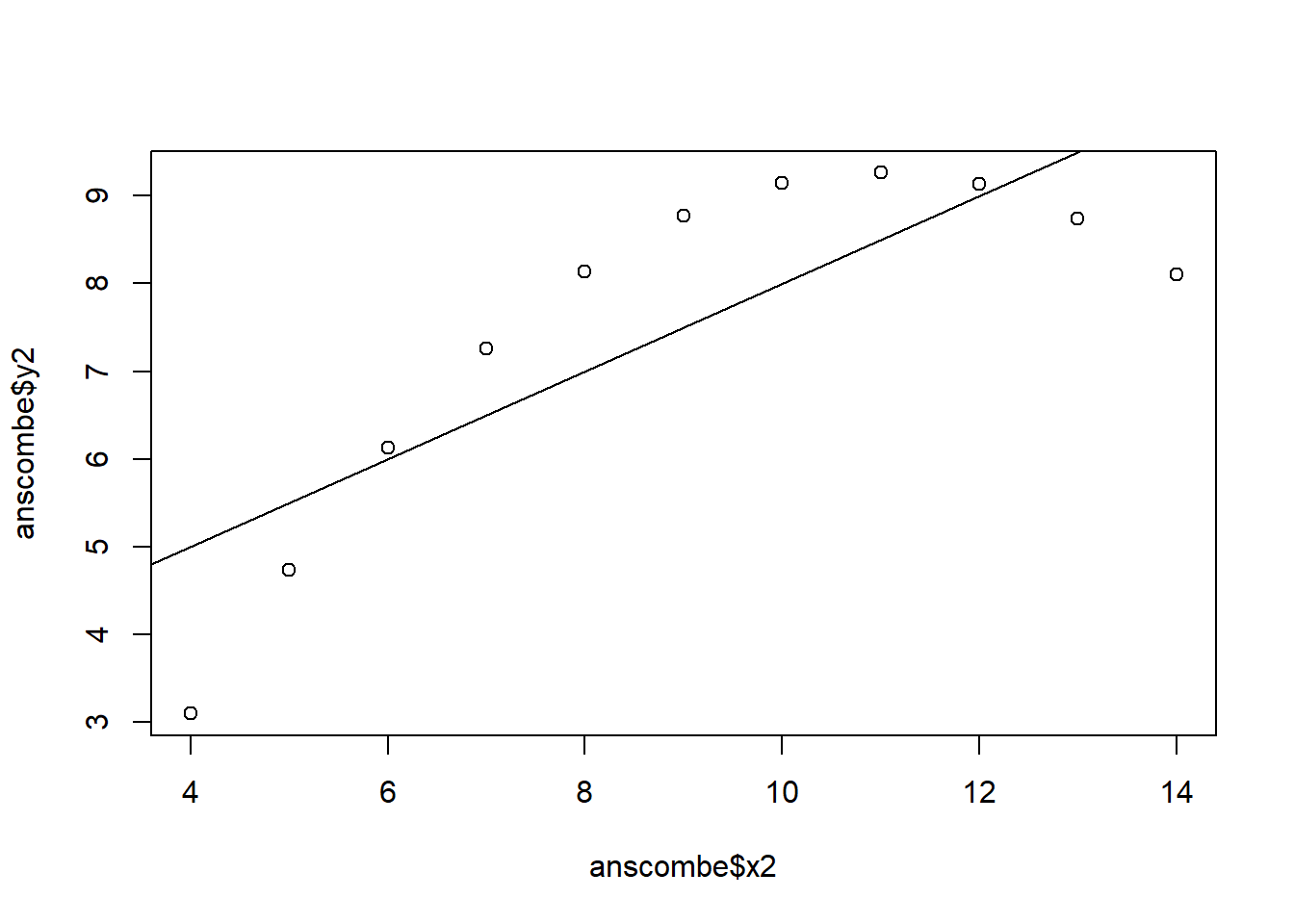
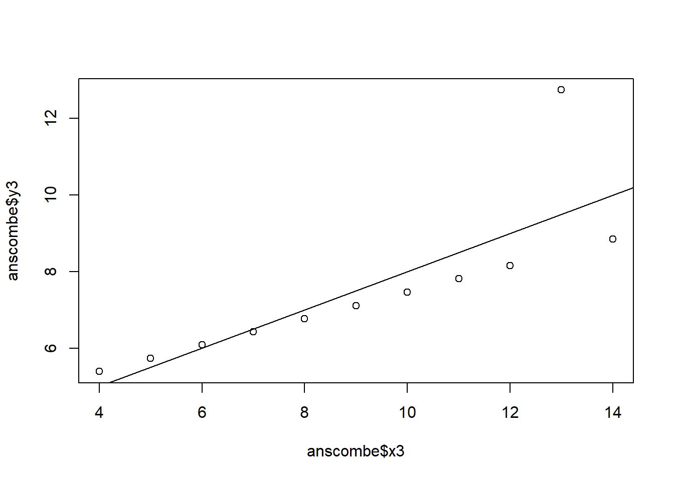
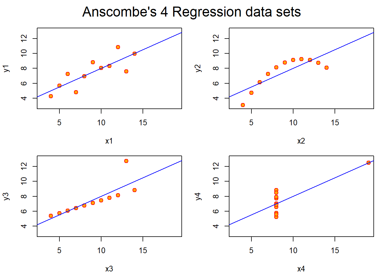
In this example, the linear regression line is the same for all the models and yet, their scatter plot tells us that there is a better option to fit the data.
       x1             x2             x3             x4           y1
 Min.   : 4.0   Min.   : 4.0   Min.   : 4.0   Min.   : 8   Min.   : 4.260
 1st Qu.: 6.5   1st Qu.: 6.5   1st Qu.: 6.5   1st Qu.: 8   1st Qu.: 6.315
 Median : 9.0   Median : 9.0   Median : 9.0   Median : 8   Median : 7.580
 Mean   : 9.0   Mean   : 9.0   Mean   : 9.0   Mean   : 9   Mean   : 7.501
 3rd Qu.:11.5   3rd Qu.:11.5   3rd Qu.:11.5   3rd Qu.: 8   3rd Qu.: 8.570
 Max.   :14.0   Max.   :14.0   Max.   :14.0   Max.   :19   Max.   :10.840
       y2              y3              y4
 Min.   :3.100   Min.   : 5.39   Min.   : 5.250
 1st Qu.:6.695   1st Qu.: 6.25   1st Qu.: 6.170
 Median :8.140   Median : 7.11   Median : 7.040
 Mean   :7.501   Mean   : 7.50   Mean   : 7.501
 3rd Qu.:8.950   3rd Qu.: 7.98   3rd Qu.: 8.190
 Max.   :9.260   Max.   :12.74   Max.   :12.500
```
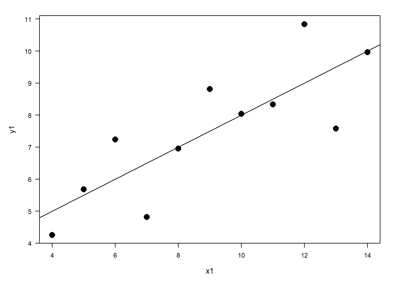
For y1 ~ x1, the linear regression line seems to be a good fit for the model.
For y2 ~ x2, a quadratic regression line seems to be a better fit.
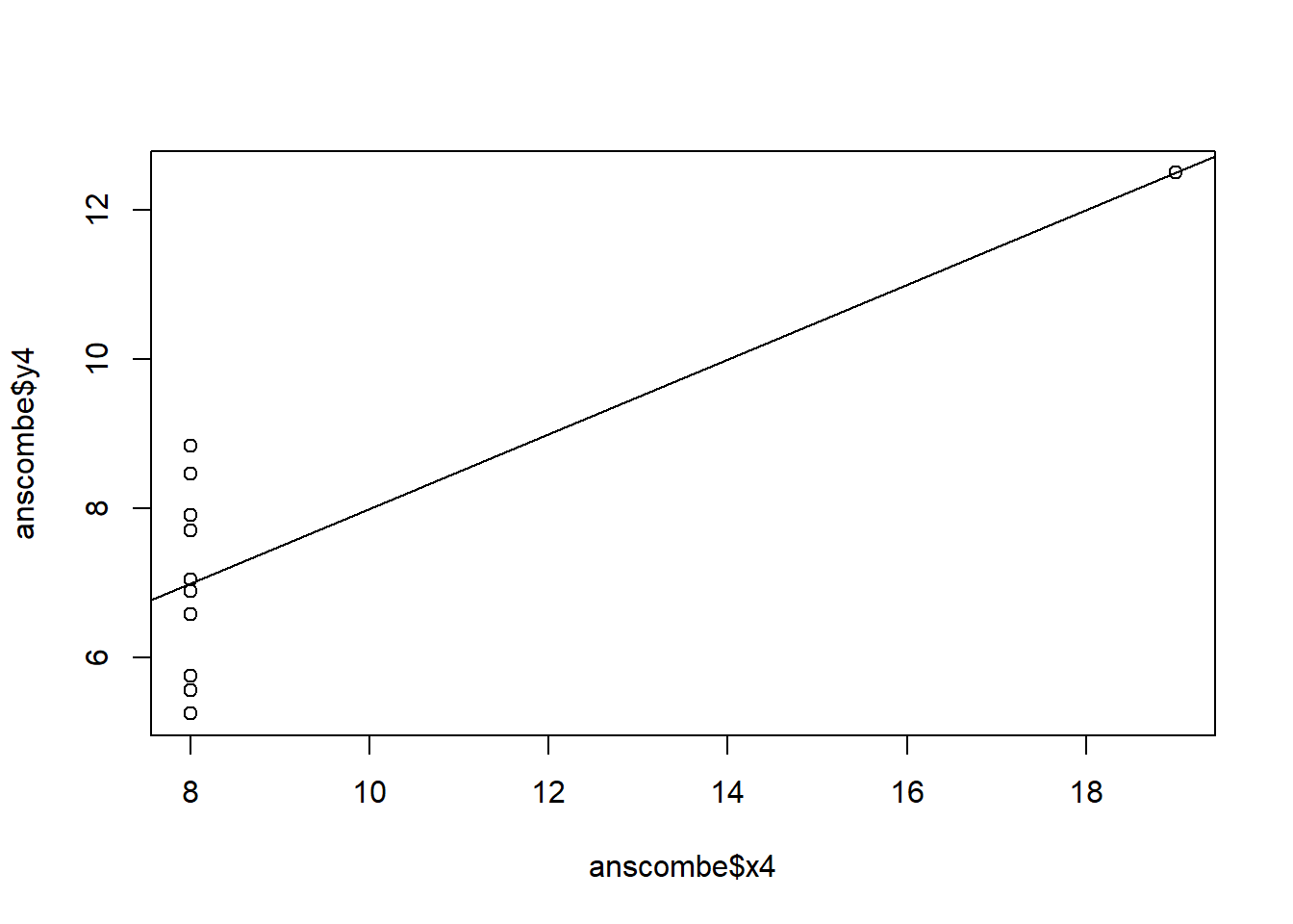
For y3 ~ x3 and y4 ~ x4, we might consider discarding the last data point as an outlier.
Call:
lm(formula = y1 ~ x1, data = anscombe)

Residuals:
     Min       1Q   Median       3Q      Max
-1.92127 -0.45577 -0.04136  0.70941  1.83882

Coefficients:
            Estimate Std. Error t value Pr(>|t|)
(Intercept)   3.0001     1.1247   2.667  0.02573 *
x1            0.5001     0.1179   4.241  0.00217 **
---
Signif. codes:  0 '***' 0.001 '**' 0.01 '*' 0.05 '.' 0.1 ' ' 1

Residual standard error: 1.237 on 9 degrees of freedom
Multiple R-squared:  0.6665,    Adjusted R-squared:  0.6295
F-statistic: 17.99 on 1 and 9 DF,  p-value: 0.00217
Call:
lm(formula = y2 ~ x2, data = anscombe)

Residuals:
    Min      1Q  Median      3Q     Max
-1.9009 -0.7609  0.1291  0.9491  1.2691

Coefficients:
            Estimate Std. Error t value Pr(>|t|)
(Intercept)    3.001      1.125   2.667  0.02576 *
x2             0.500      0.118   4.239  0.00218 **
---
Signif. codes:  0 '***' 0.001 '**' 0.01 '*' 0.05 '.' 0.1 ' ' 1

Residual standard error: 1.237 on 9 degrees of freedom
Multiple R-squared:  0.6662,    Adjusted R-squared:  0.6292
F-statistic: 17.97 on 1 and 9 DF,  p-value: 0.002179
Call:
lm(formula = y3 ~ x3, data = anscombe)

Residuals:
    Min      1Q  Median      3Q     Max
-1.1586 -0.6146 -0.2303  0.1540  3.2411

Coefficients:
            Estimate Std. Error t value Pr(>|t|)
(Intercept)   3.0025     1.1245   2.670  0.02562 *
x3            0.4997     0.1179   4.239  0.00218 **
---
Signif. codes:  0 '***' 0.001 '**' 0.01 '*' 0.05 '.' 0.1 ' ' 1

Residual standard error: 1.236 on 9 degrees of freedom
Multiple R-squared:  0.6663,    Adjusted R-squared:  0.6292
F-statistic: 17.97 on 1 and 9 DF,  p-value: 0.002176
Call:
lm(formula = y4 ~ x4, data = anscombe)

Residuals:
   Min     1Q Median     3Q    Max
-1.751 -0.831  0.000  0.809  1.839

Coefficients:
            Estimate Std. Error t value Pr(>|t|)
(Intercept)   3.0017     1.1239   2.671  0.02559 *
x4            0.4999     0.1178   4.243  0.00216 **
---
Signif. codes:  0 '***' 0.001 '**' 0.01 '*' 0.05 '.' 0.1 ' ' 1

Residual standard error: 1.236 on 9 degrees of freedom
Multiple R-squared:  0.6667,    Adjusted R-squared:  0.6297
F-statistic:    18 on 1 and 9 DF,  p-value: 0.002165
Analysis of Variance Table

Response: y1
          Df Sum Sq Mean Sq F value  Pr(>F)
x1         1 27.510 27.5100   17.99 0.00217 **
Residuals  9 13.763  1.5292
---
Signif. codes:  0 '***' 0.001 '**' 0.01 '*' 0.05 '.' 0.1 ' ' 1
Analysis of Variance Table

Response: y2
          Df Sum Sq Mean Sq F value   Pr(>F)
x2         1 27.500 27.5000  17.966 0.002179 **
Residuals  9 13.776  1.5307
---
Signif. codes:  0 '***' 0.001 '**' 0.01 '*' 0.05 '.' 0.1 ' ' 1
Analysis of Variance Table

Response: y3
          Df Sum Sq Mean Sq F value   Pr(>F)
x3         1 27.470 27.4700  17.972 0.002176 **
Residuals  9 13.756  1.5285
---
Signif. codes:  0 '***' 0.001 '**' 0.01 '*' 0.05 '.' 0.1 ' ' 1
Analysis of Variance Table

Response: y4
          Df Sum Sq Mean Sq F value   Pr(>F)
x4         1 27.490 27.4900  18.003 0.002165 **
Residuals  9 13.742  1.5269
---
Signif. codes:  0 '***' 0.001 '**' 0.01 '*' 0.05 '.' 0.1 ' ' 1
$lm1
             Estimate Std. Error  t value    Pr(>|t|)
(Intercept) 3.0000909  1.1247468 2.667348 0.025734051
x1          0.5000909  0.1179055 4.241455 0.002169629

$lm2
            Estimate Std. Error  t value    Pr(>|t|)
(Intercept) 3.000909  1.1253024 2.666758 0.025758941
x2          0.500000  0.1179637 4.238590 0.002178816

$lm3
             Estimate Std. Error  t value    Pr(>|t|)
(Intercept) 3.0024545  1.1244812 2.670080 0.025619109
x3          0.4997273  0.1178777 4.239372 0.002176305

$lm4
             Estimate Std. Error  t value    Pr(>|t|)
(Intercept) 3.0017273  1.1239211 2.670763 0.025590425
x4          0.4999091  0.1178189 4.243028 0.002164602
## 2. Fine tune the charts with RGraphics by Murrell
## 3. Fine tune the charts with ggplot
Source Code
---title: "Assignment 3"author: "Vikrant Sagar R"date: "2022-09-24"categories: [Code, R, Plots, Assignment]draft: falseformat: html: code-fold: true code-tools: trueexecute: echo: false---\## 1. Explore Anscombe (1973) QuartletIn this example, the linear regression line is the same for all the models and yet, their scatter plot tells us that there is a better option to fit the data.```{r}#| echo: false#| fig-cap: "Simple Model"## Anscombe (1973) Quartletrm(list=ls())data(anscombe) # Load Anscombe's data## Simple versionplot(anscombe$x1,anscombe$y1)summary(anscombe)```\`\`\`For y1 \~ x1, the linear regression line seems to be a good fit for the model.For y2 \~ x2, a quadratic regression line seems to be a better fit.For y3 \~ x3 and y4 \~ x4, we might consider discarding the last data point as an outlier.```{r}#| echo: false#| output: false#| fig-cap: "Four Model Objects"#| fig-subcap:#| - "y1 ~ x1"#| - "y2 ~ x2"#| - "y3 ~ x3"#| - "y4 ~ x4"#| layout-ncol: 2#| layout-nrow: 2# Create four model objectslm1 <-lm(y1 ~ x1, data=anscombe)summary(lm1)lm2 <-lm(y2 ~ x2, data=anscombe)summary(lm2)lm3 <-lm(y3 ~ x3, data=anscombe)summary(lm3)lm4 <-lm(y4 ~ x4, data=anscombe)summary(lm4)plot(anscombe$x1,anscombe$y1)abline(coefficients(lm1))plot(anscombe$x2,anscombe$y2)abline(coefficients(lm2))plot(anscombe$x3,anscombe$y3)abline(coefficients(lm3))plot(anscombe$x4,anscombe$y4)abline(coefficients(lm4))``````{r}#| echo: false## Fancy version (per help file)ff <- y ~ xmods <-setNames(as.list(1:4), paste0("lm", 1:4))# Plot using for loopfor(i in1:4) { ff[2:3] <-lapply(paste0(c("y","x"), i), as.name)## or ff[[2]] <- as.name(paste0("y", i))## ff[[3]] <- as.name(paste0("x", i)) mods[[i]] <- lmi <-lm(ff, data = anscombe)print(anova(lmi))}sapply(mods, coef) # Note the use of this functionlapply(mods, function(fm) coef(summary(fm)))# Preparing for the plotsop <-par(mfrow =c(2, 2), mar =0.1+c(4,4,1,1), oma =c(0, 0, 2, 0))# Plot charts using for loopfor(i in1:4) { ff[2:3] <-lapply(paste0(c("y","x"), i), as.name)plot(ff, data = anscombe, col ="red", pch =21, bg ="orange", cex =1.2,xlim =c(3, 19), ylim =c(3, 13))abline(mods[[i]], col ="blue")}mtext("Anscombe's 4 Regression data sets", outer =TRUE, cex =1.5)par(op)```\## 2. Fine tune the charts with RGraphics by Murrell```{r}#| echo: false#| fig-cap: "x1 ~ y1 Chart fine-tuned with RGraphics by Murrell"par(las=1, mar=c(5, 5, 2, 2), cex=.7) plot.new()plot.window(range(anscombe$x1), c(0, 6))plot(anscombe$x1,anscombe$y1, ylab ="", xlab ="")points(anscombe$x1,anscombe$y1, pch=16, cex=2)abline(coefficients(lm1))mtext("x1", side=1, line=3, cex=0.8)mtext("y1", side=2, line=3, las=0, cex=0.8)```\## 3. Fine tune the charts with ggplot```{r}#| echo: false#| fig-cap: "x1 ~ y1 Chart fine-tuned with ggplot2"library(ggplot2)ggplot(anscombe, aes(x1, y1)) +geom_point()+geom_line()```